Ancestral Sequence Reconstruction

Ancestral Sequence Reconstruction

Introduction

What is an Ancestral Sequence Reconstruction?

Ancestral Sequence Reconstruction (ASR) is a technique where extant protein or DNA sequences are used to infer what the common ancestor mighth have looked like. It is a bit of a protein time machine that guesses the most likely trajectory of evolution only from what we see in the present. So let’s say for example you have some protein family that exhibitis two different functions amongst its members: breaking down a substrate and using it as a co-substrate for a reaction. With ASR you could find out which of the two functions came first by inferring the ancestral sequence followed by screening in the lab. This can be quite useful, because you can for example resurrect the ancient receptor that lies at the base of a receptor family. By using this ancestor as a target you can potentially create a protein that binds all extant members of the protein family.

What goes into an ASR

Any ASR starts of with a set of sequences of which you want an ancestor. All sequences have to be related otherwise they would not share an ancestor. Also guessing the evolutionary trajectory is not a benign task and therefore gets more and more uncertain the further you go back in time. You are more likely to succeed the more recent the ancestor you want to reconstruct is. Also you will need outgroup sequences which are very closely related to guess the changes that happened leading up to the ancestor you want to create.

How does it does it work?

The basic principle behind an ASR is to look at all sequences in the dataset on a site per site basis and try to trace back changes through the family tree of the protein. For one single base the principle is illustrated below where we have Function 1 and 2 belonging to one protein family and we want to know what the ancestor of this protein family looks like. Here we only consider a singular site which would need to be repeated for all sites in a proper ASR.

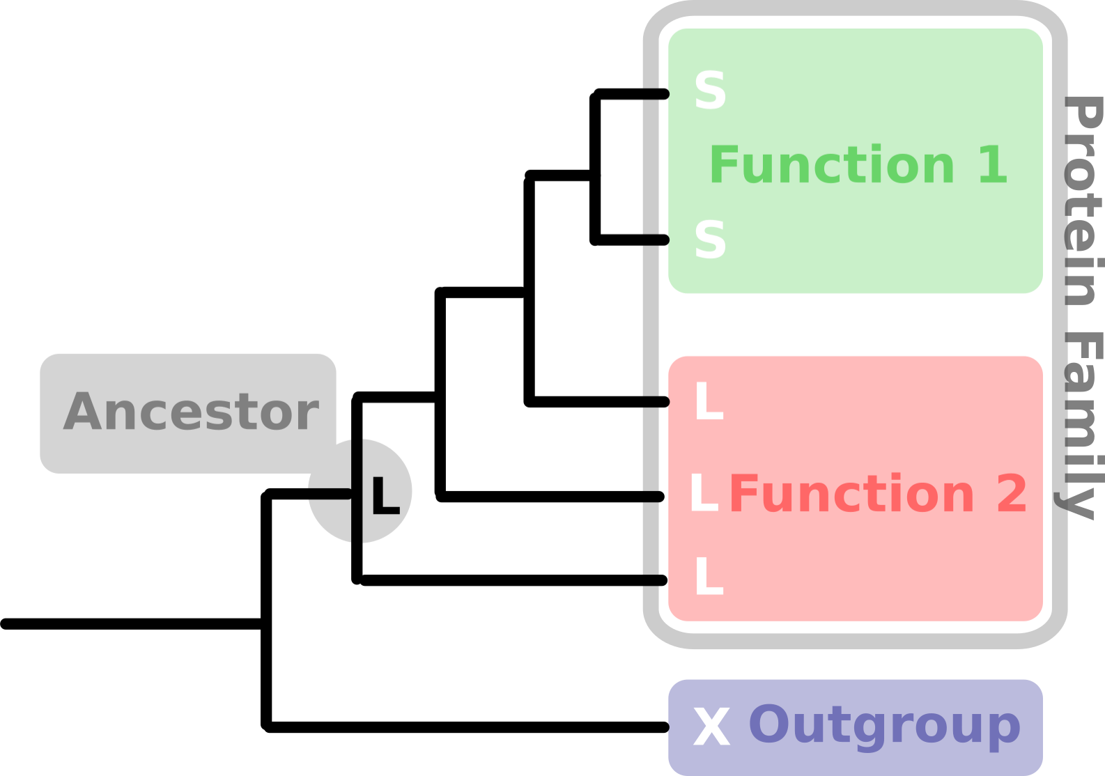
Just from one amino acid it would look like the ancestor of this protein family would exhibit function 2. This is a very simplified version of the underlying principle and as there are a lot of sequences and a lot of sites involved in the process, there is a fair amount of statistics going into an ASR. So where do we begin?

Materials and Methods

Which program to use?

There are multiple ways to reconstruct a sequence and there are different opinions out there as to which is the best. This highly depends on your sequences and what purpose you are doing an ASR for. One path which is very easy to follow and still creates really good results which is using Mega X. Mega stands for Molecular Evolutionary Genetics Analysis and is the swiss army knife of sequence analysis and I encourage you to check out the different features in the manual. Mega, which you can get from here, can take you the full way from sequences to ancestral reconstruction without ever closing the program once. So now we have a program of choice we need to choose a dataset next.

Dataset collection

Collecting a dataset of the protein family of interest is always a bit of a trade-off. You need to include as many sequences as possible to give a wide variety of different proteins that represent all the functions you are interested in. However, including too many sequences will lead to immense computational requirements and thus calculation times. Ideally you would be looking at a phylogenetic tree of all sequences within the protein family and a few of the closest relatives (for a touch up on how to do phylogenetic trees check this report. From here you need to locate the node which corresponds to the base of the protein family you are interested in. Sequences that branch off immediately after and before the node you want to reconstruct are the most important for your analysis. Those sequences are most influential on what your ancestor looks like. In general also your dataset would need to include a good variety of different sequences within the protein family. Theoretically you can input an infinite amount of sequences into your reconstruction, however to keep the dataset manageable it’d be good to have about 100-200 sequences. This will also require you to have decent computer with let’s say about 8 virtual cores at least (check out this report for an explanation of computer architecture)

Once you have collected your sequences can start aligning for which you need to store everything in one fasta file (for a quick primer on the fasta format check this report).

Sequence Alignment

First you would need to open your fasta file using the menu in the upper left corner of your screen. Click File>Open A File and select the fasta file with your sequences. Mega will ask you to align or analyze the sequences, here select align. This will open a new window where you can see your sequence coloured by the different amino acids. You will quickly realise by the jumble of colours that this is not at all a viable alignment. This is because Mega hasn’t actually aligned them yet but rather put them in an alignment viewer.

From here navigate to Alignment>Align with ClustalW. There will be a lot of parameters like gap opening and gap extension penalties which is the program asking you how likely you think insertions and deletions are. If you do not know exactly what you are doing it is a good idea to stick with defaults. Hopefully it will look a lot less messy now. Here you can also gage whether you are likely to have selected sequences which are similar enough to get an ancestor from. If your alignment is full of gaps ( the “-“ character) it means that your sequences are too distant and the algorithm can not figure out which sites have the same evolutionary origin (homologous sites). If this is the case you would need to rethink your whole dataset. Maybe exclude a few very distant sequences one by one and recheck your alignment. If your alignment looks like mine below you are doing pretty well.

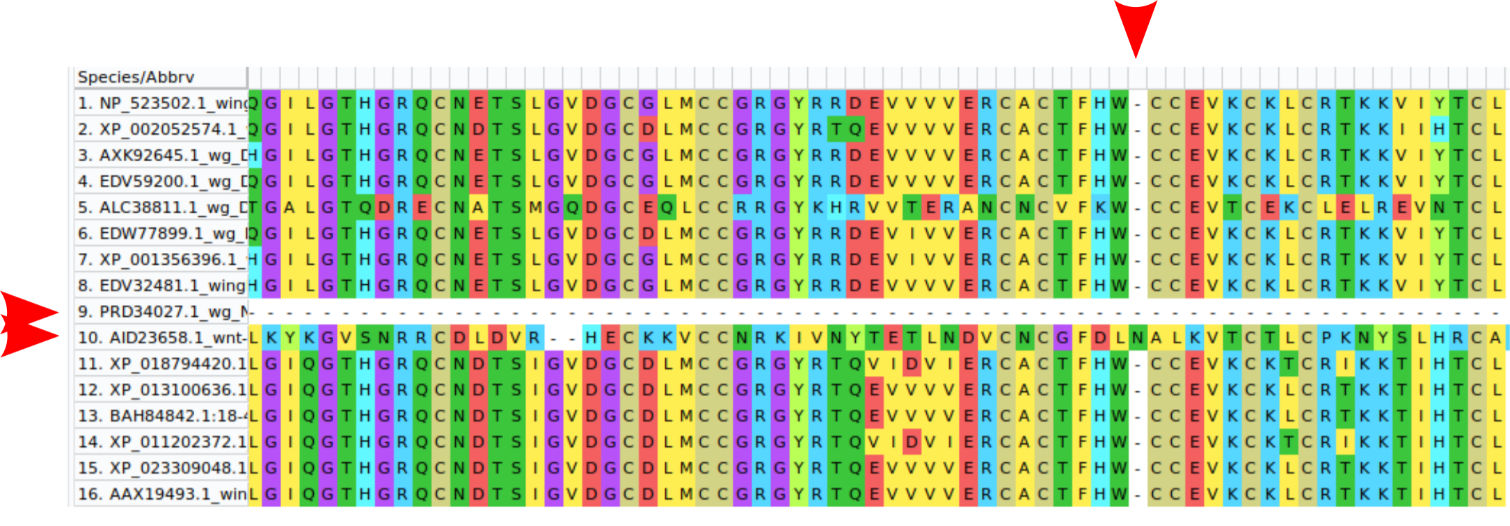
As often in science pretty good is not good enough. There is one column that I highlighted with a red arrow that can be deleted only one sequence has an additional amino acid which is unlikely to be present in the ancestor. I also highlighted two rows which either contain no information (all gaps) or are seemingly a protein which doesn’t belong to this family (completely misaligned) which I would also delete. We are in the process of manually curating an alignment which requires a lot of decision making and a bit of experience. If unsure about how to curate an alignment ask someone who is more experienced or simply trust the algorithms. Once your alignment looks good you can continue with your phylogenetic tree construction. Now to save the alignment click on Data>Export Alignment>MEGA Format and save it.

Substitution Model

Before you can construct a tree, you will need to find out which substitution model fits your data best. A substitution model tries to quantify how frequently one amino acid (or nucleotide) changes to another from the data you present it. The assumption is that more frequent changes are more likely and thus need less time to evolve. Two sequences exhibiting more likely changes should be closer together in a tree than two sequences exhibiting only very unlikely changes. There are a good number of substitution models out there and you don’t need to now them all, you just need to know which one suits your data best. I would keep all options as is in the pop-up window. The number of threads option on the bottom shows you how many times this operation should be run in parallel on your computer. Mega will set it automatically to the number of your virtual cores -1 which is a good choice. Once you have run this analysis a table will pop up. The substitution model at the top should be the one you specify for the tree construction. The different columns in the tree are different ways to estimate how likely the substitution model is for your data (BIC = Bayesian information criterion, AIC = Akaike information criterion). This is also not really relevant for you to know but good to note down in a report to show that you have determined an optimal substitution model.

Phylogenetic Tree

Locate the Phylogeny button on the upper border of your Mega window, click Construct Maximum Likelihood tree and open the alignment file you just created. Here we will establish what the most likely underlying phylogenetic relationship between our sequences is ( for a quick brush up on what maximum likelihood is check out this report). The pop-up window will give you the option “Test of Phylogeny” where you have the option of None and Bootstrap method. In bootstrapping you try to establish how robust your estimation is to noise, which is done by subsampling with replacement. If you alignment has, for example, 100 residues (the columns of your alignment) you throw them all in a hat. Now you will draw 100 residues at random from that hat one after the other. Whenever you draw a residue from the hat it will be replaced and can be drawn again. This will lead to some residues (columns) being drawn multiple times and some never being drawn, which introduces some noise into your estimation. Every time you pick 100 residues you have created one bootstrap replicate. The default in Mega is 50 replicates meaning that you will draw 50 alignments each slightly different from the original alignment. If the majority of the replicates agree on a node in the phylogeny, we consider this node to be fairly robust to noise. We now have some estimation whether we should trust that node. In practice this would lead to “collapsing” nodes which have less than 50% bootstrap replicates support (this value is arbitrary and depends on your choice). Collapsing a node will add the branches coming from that node to the parent node (leading to nodes with 3 or more branches which is called a politomy). Collapsing a node with weak bootstrap support is better than keeping it in a way that it is better to admit to know nothing than to pretend to know something when you don’t. Under the Model you should choose the substitution model you have estimated in the previous step. If it had a +G, +I or +GI character at the you should specify that under Rates among sites. This defines how the substitution model can change among different residues. I would leave the rest of the options as is.

The result will be a phylogenetic tree with bootstrap support shown next to the nodes. The length of the branches should correspond to evolutionary distance between the sequences, which was established using the substitution model from the previous step. Here you can check whether your tree makes sense, meaning that your outgroup sequences and all members of your protein family are grouped together respectively. Now you can finally reconstruct ancestors. Export the current tree under File>Export Current Tree(Newick).

Ancestor Reconstruction

In the main window of Mega click on Ancestors and choose the Mega file of your alignment, then under tree to use select the newick tree you just saved. Under Model and Rates among sites specify the same options as you have chosen for the phylogenetic tree. Under Gaps you could choose to completely ignore gaps or only consider the sequences that are present, which depends on what your alignment looks like. If you use all sites the ancestor could exhibit a gap as ancestral state which would mean there was an insertion after the ancestor. I would recommend to leave everything as is for now.

Once computed the ASR will again give you a phylogenetic tree, however now it will display characters at every node in the tree. This character corresponds to what the algorithm thinks was most likely present in the ancestor corresponding to this node. In the upper right corner you can cycle through the different positions of your sequence. If the algorithm is not sure which amino acid to place it will display all the characters that are possible.

A more comprehensive overview can be generated by selecting Ancestors>Export most probable sequences. This will give you an excel file which shows the most likely amino acid at every position in the tree. The row names correspond to the different sequence headers followed by the nodes of the tree which are numbered. You can check which number corresponds to which node under View>Show/Hide>Node IDs. Now you just have to locate the node of your ancestor of interest for example the node connecting every member of the protein family you are looking at. The row in the excel table corresponding to this number will then show you what the ancestral sequence is. Be aware however, that the probabilities of each amino acid are marked in colour and red cells indicate that the algorithm is not very sure which amino acid to pick. Here it gets very difficult and you would need a bit of background knowledge to pick the right one. Sometimes this can be determined by looking at the structure of the protein and establishing which amino acid makes the most sense. Like, for example, a prolin in the middle of a helix would be pretty detrimental to structure. If unsure just leave red cells as they are. Hopefully there are not too many red cells and you have now successfully reconstructed an ancestral protein. Congratulations!

Written by Nicolas Arning